---
title: "Visualizing Pell Grant Awards in the U.S. in 2017"
description: "Exploring Colorado trends and the overall state-level Pell grant distribution"
author:
- name: Mickey Rafa
url: https://mrafa3.github.io/
date: 12-30-2022
categories: [R, "#TidyTuesday", line-plot, gt] # self-defined categories
image: "tt_2022_35_thumbnail.png"
draft: false # setting this to `true` will prevent your post from appearing on your listing page until you're ready!
format:
html:
toc: true
toc-depth: 5
code-link: true
code-fold: true
code-tools: true
code-summary: "Show code"
self-contained: true
editor_options:
chunk_output_type: inline
execute:
error: false
message: false
warning: false
eval: true
---
{#fig-1}
{#fig-1}
# 1. Load Packages & Setup
```{r setup, include=TRUE}
if (!require("pacman")) install.packages("pacman")
pacman::p_load(
    tidyverse,
    tidytuesdayR,
    dlookr,
    ggtext,
    gt,
    gtExtras,  #for font awesome icons in gt tables
    ggbump,
    showtext,
    janitor,   #for clean_names()
    scales,
    htmltools, #for tagList()
    glue,
    epoxy,
    here,
    geomtextpath
)

font_add('fa-brands', 'fonts/Font Awesome 6 Brands-Regular-400.otf')
sysfonts::font_add_google("Lato","lato")
showtext::showtext_auto()
```
# 2. Read in the Data
```{r read_data, include=TRUE}
tt_year <- 2022
tt_week <- 35

tuesdata <- tidytuesdayR::tt_load(tt_year, week = tt_week)

df <- tuesdata$pell %>%
  clean_names()
```
# 3. Examine the Data
```{r examine, include=TRUE, echo=TRUE}
df %>%
  glimpse()
```
# 4. Tidy the Data
```{r tidy_pell, include=TRUE}
df_colorado <- df %>%
  filter(state == 'CO') %>%
  mutate(award_per_recipent = award / recipient)

df_colorado_min <- df_colorado %>%
  filter(recipient >= 10) %>%
  group_by(year) %>%
  slice_min(award_per_recipent) %>%
  mutate(min_max_label = 'Min')

df_colorado_max <- df_colorado %>%
  filter(recipient >= 10) %>%
  group_by(year) %>%
  slice_max(award_per_recipent) %>%
  mutate(min_max_label = 'Max')

df_colorado_min_max <- bind_rows(df_colorado_min, df_colorado_max)
```
```{r df_tbl, include=TRUE}
df_tbl <- df %>%
  slice_max(year) %>%
  group_by(state) %>%
  summarise(sum_award = sum(award, na.rm = TRUE),
            sum_recipients = sum(recipient, na.rm = TRUE)) %>%
  ungroup() %>%
  mutate(award_per_recipient = sum_award / sum_recipients) %>%
  arrange(-award_per_recipient)
```
# 5. Visualization Parameters
```{r my_theme, include=TRUE}
my_theme <- theme(
text = element_text(family = 'Lato', size=14, color='black'),
# plot.title = element_textbox_simple(color="black", face="bold", size=20, hjust=0),
# plot.subtitle = element_textbox_simple(color="black", size=12, hjust=0),
#axis.title = element_blank(),
#axis.text = element_blank(),
axis.ticks = element_blank(),
#axis.line = element_blank(),
# plot.caption = element_textbox_simple(color="black", size=12),
panel.background = element_blank(),
panel.grid.major = element_blank(),
panel.grid.minor = element_blank(),
panel.border = element_blank(),
legend.position = 'none')
txt <- 'black'
twitter <- glue("<span style='font-family:fa-brands; color:{txt}'></span>")
github <- glue("<span style='font-family:fa-brands; color:{txt}'></span>")
space <- glue("<span style='color:black;font-size:1px'>'</span>")
viz_colors <- c('Max' = '#645A7B', 'Min' = '#6ED187')
title_text <- 'Pell Grant Award Value per Recipient'
subtitle_text <- glue("<span style='color:#6ED187'>Min</span> and <span style='color:#645A7B'>Max</span> values each year in Colorado")
caption_text <- glue("Tidy Tuesday Week 35 (2022)<br>{twitter} @mickey.rafa • {github} mrafa3")
max_value <- df_colorado_min_max %>%
filter(year == 2010,
min_max_label == 'Max') %>%
pull(award_per_recipent)
```
# 6. Plot
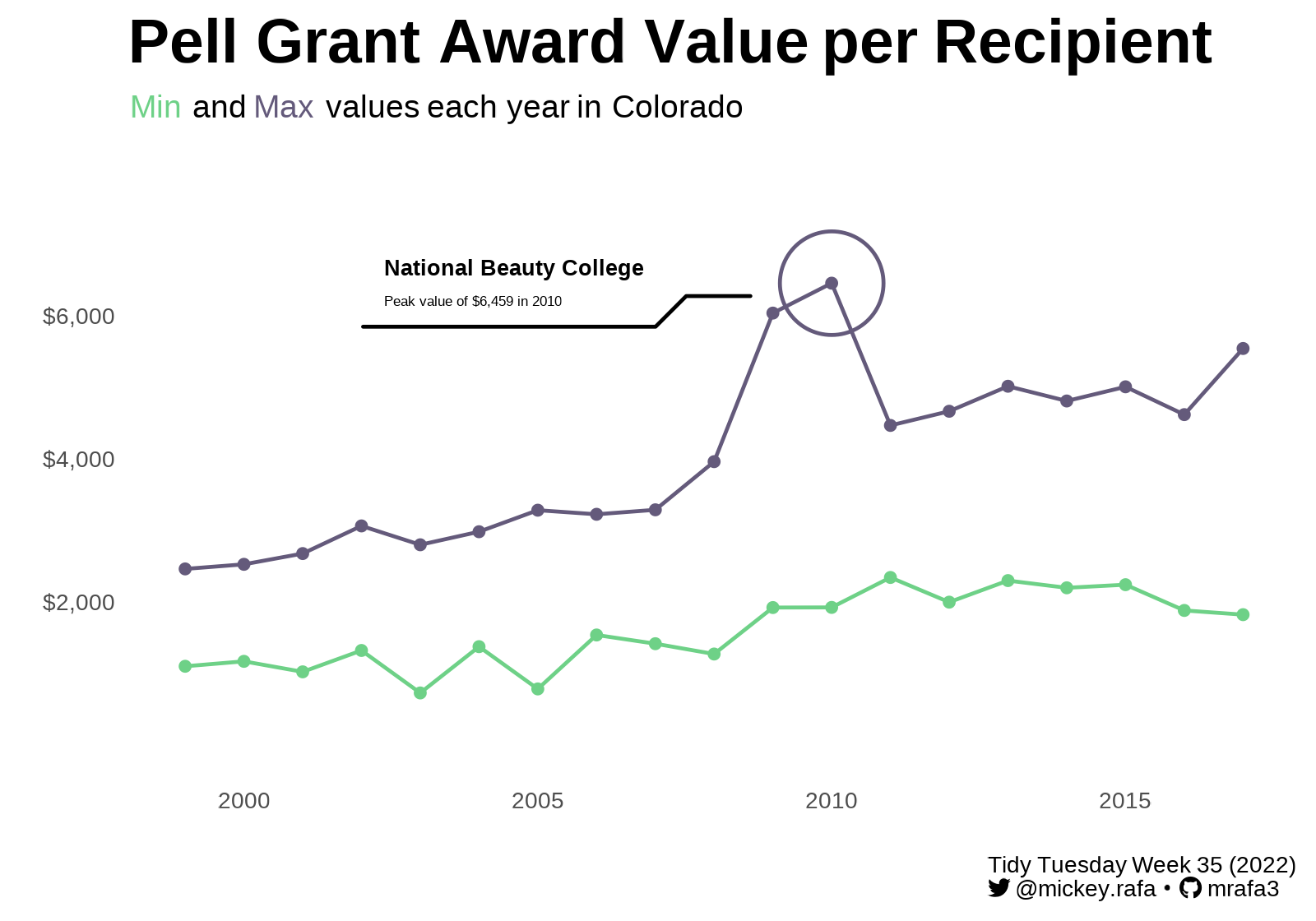
#### What is the overall trend in Pell grant awards in Colorado?
```{r viz_pell_colorado, include=TRUE}
viz_pell_colorado <- df_colorado_min_max %>%
  ggplot(.,
         aes(x=year,
             y=award_per_recipent,
             color=min_max_label)) +
  geom_point(size=1) +
  geom_line() +
  ggforce::geom_mark_circle(aes(filter = year == 2010 & min_max_label == 'Max',
                                label = name,
                                description = epoxy("Peak value of {.dollar round(max_value, 0)} in 2010")),
                            label.family = 'Lato',
                            label.fontsize = c(20, 13)) +
  labs(x='',
       y='',
       title = title_text,
       subtitle = subtitle_text,
       caption = caption_text) +
  scale_y_continuous(labels = c('', '$2,000', '$4,000', '$6,000', ''),
                     limits = c(0,8000)) +
  scale_color_manual(values = viz_colors) +
  my_theme +
  theme(plot.title = element_textbox(size=rel(4), face='bold'),
        plot.subtitle = element_textbox(size=rel(2.1)),
        plot.caption = element_textbox(size=rel(1.5), lineheight=.3),
        axis.text = element_text(size=rel(1.5)))
```
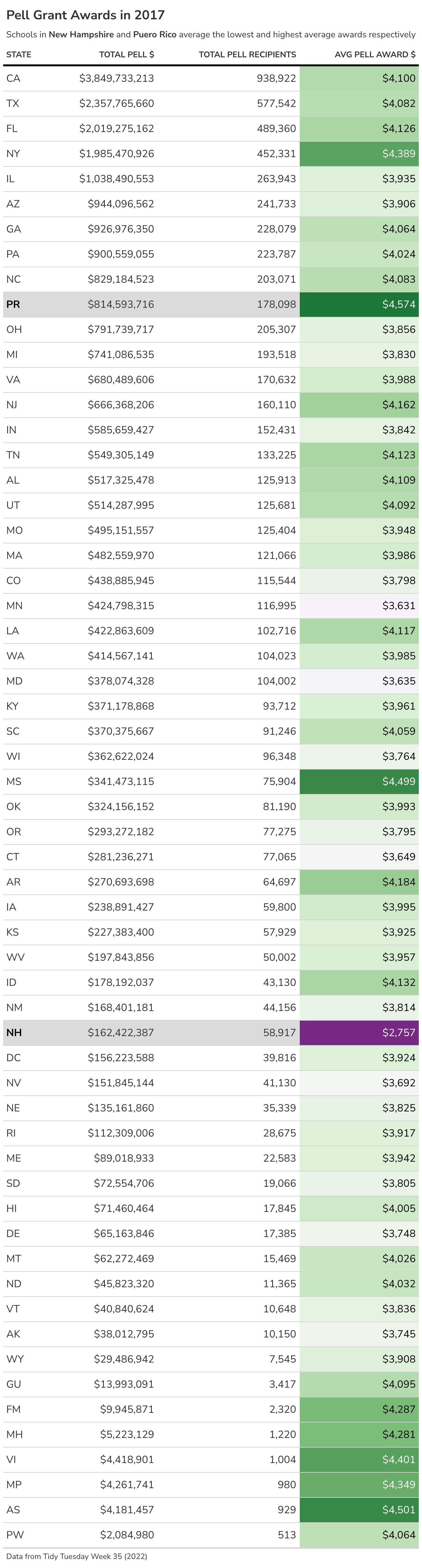
#### Which state has the highest pell award per student?
```{r tbl_viz, include=TRUE}
tbl_viz <- df_tbl %>%
  arrange(-sum_award) %>%
  gt() %>%
  gt::cols_label(state = 'State',
                 sum_award = 'Total Pell $',
                 sum_recipients = 'Total Pell Recipients',
                 award_per_recipient = 'Avg Pell Award $') %>%
  tab_header(title = md("**Pell Grant Awards in 2017**"),
             subtitle = md("Schools in **New Hampshire** and **Puero Rico** average the lowest and highest average awards respectively")) %>%
  tab_source_note(source_note = "Data from Tidy Tuesday Week 35 (2022)") %>%
  fmt_currency(columns = c(sum_award, award_per_recipient),
               decimals = 0) %>%
  fmt_number(columns = c(sum_recipients),
               decimals = 0) %>%
  gt_highlight_rows(
    rows = c(10,39),
    fill = "lightgrey",
    bold_target_only = TRUE,
    target_col = state
    ) %>%
  gt_hulk_col_numeric(award_per_recipient) %>%
  tab_style(
    locations = cells_column_labels(columns = everything()),
    style = list(
      #thick border
      cell_borders(sides = "bottom", weight = px(3)),
      #make text bold
      cell_text(weight = "bold")
    )
  ) %>%
  #apply different style to title
  tab_style(locations = cells_title(groups = "title"),
            style = list(
              cell_text(weight = "bold", size = 24)
            )) %>%
  opt_all_caps() %>%
  opt_table_font(
    font = list(
      google_font("Nunito Sans"),
      default_fonts()
    )
  ) %>%
  tab_options(
    #remove border between column headers and title
    column_labels.border.top.width = px(3),
    column_labels.border.top.color = "transparent",
    #remove border around the table
    table.border.top.color = "transparent",
    table.border.bottom.color = "transparent",
    #adjust font sizes and alignment
    source_notes.font.size = 12,
    heading.align = "left"
  )
```
# 7. Save
```{r save_plot, include=TRUE}
# Save the plot as PNG
ggsave(
  filename = glue("tt_{tt_year}_{tt_week}.png"),
  plot = viz_pell_colorado,
  width = 5, height = 3.5, units = "in", dpi = 320
)

tbl_viz %>%
  gtsave(
    filename = glue("tt_{tt_year}_{tt_week}_tbl.png"),
    path = here::here()
    )

# make thumbnail for page
magick::image_read(glue("tt_{tt_year}_{tt_week}.png")) %>%
  magick::image_resize(geometry = "400") %>%
  magick::image_write(glue("tt_{tt_year}_{tt_week}_thumbnail.png"))
```
# 8. Session Info
::: {.callout-tip collapse="true"}
##### Expand for Session Info
```{r, echo = FALSE}
sessionInfo()
```
:::
# 9. Github Repository
::: {.callout-tip collapse="true"}
##### Expand for GitHub Repo
[Access the GitHub repository here](https://github.com/mrafa3/mrafa3.github.io)
:::

