---
title: "Visualizing enrollment in HBCUs by gender over time"
description: "Women far outnumber men at HBCUs"
author:
- name: Mickey Rafa
url: https://mrafa3.github.io/
date: 12-21-2022
categories: [R, "#TidyTuesday", line-plot, ribbon-plot] # self-defined categories
image: "tt_2021_6_thumbnail.png"
draft: false # setting this to `true` will prevent your post from appearing on your listing page until you're ready!
format:
html:
toc: true
toc-depth: 5
code-link: true
code-fold: true
code-tools: true
code-summary: "Show code"
self-contained: true
editor_options:
chunk_output_type: inline
execute:
error: false
message: false
warning: false
eval: true
---
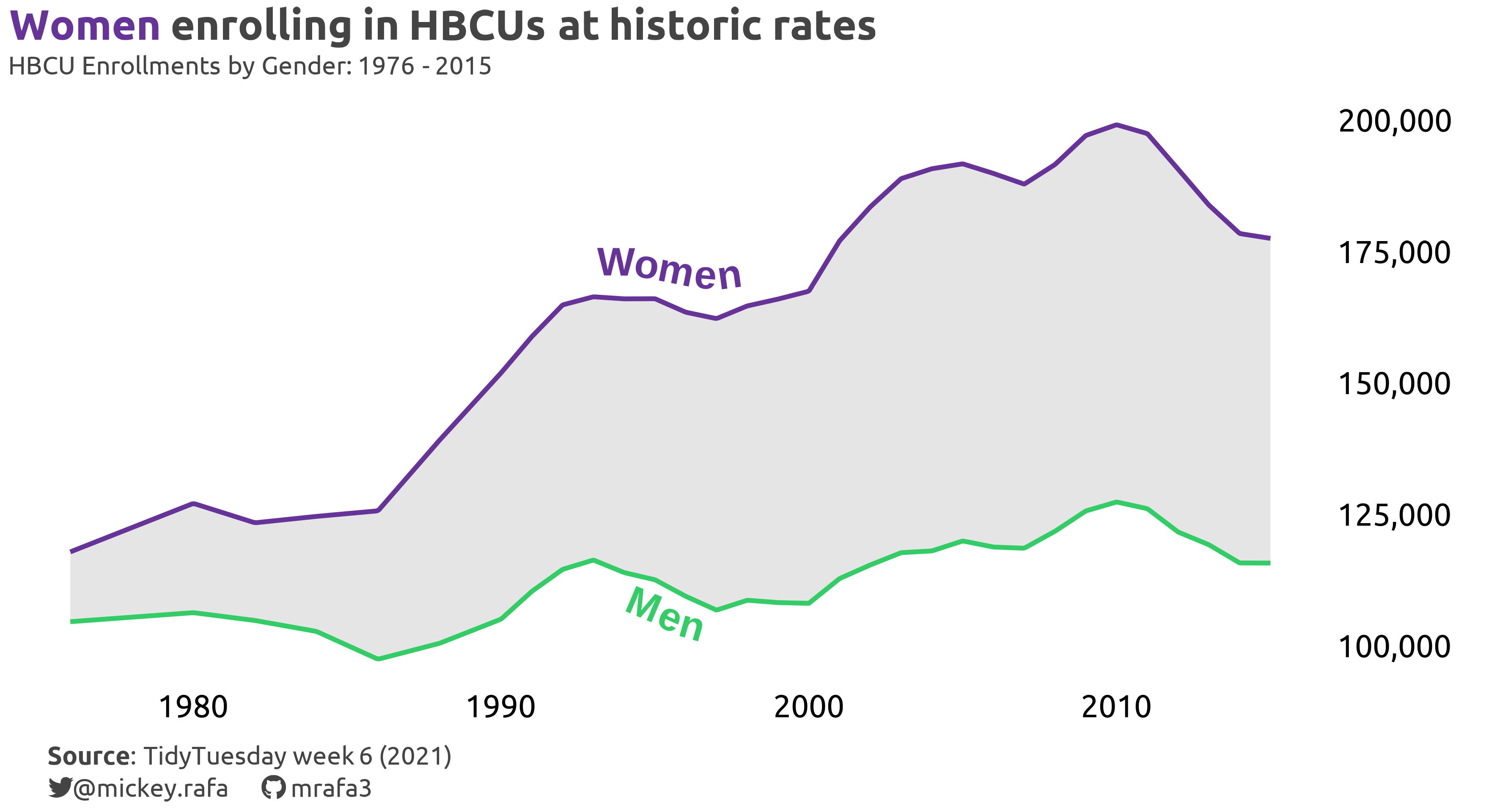{#fig-1}
# 1. Load Packages & Setup
```{r setup, include=TRUE}
if (!require("pacman")) install.packages("pacman")
pacman::p_load(
    tidyverse,
    tidytuesdayR,
    dlookr,
    ggtext,
    gt,
    gtExtras,  #for font awesome icons in gt tables
    ggbump,
    showtext,
    janitor,   #for clean_names()
    scales,
    htmltools, #for tagList()
    glue,
    here,
    geomtextpath
)

font_add('fa-reg', 'fonts/Font Awesome 6 Free-Regular-400.otf')
font_add('fa-brands', 'fonts/Font Awesome 6 Brands-Regular-400.otf')
font_add('fa-solid', 'fonts/Font Awesome 6 Free-Solid-900.otf')

sysfonts::font_add_google("Ubuntu","ubuntu")
showtext::showtext_auto()
showtext::showtext_opts(dpi=300)
```
# 2. Read in the Data
```{r read_data, include=TRUE}
tt_year <- 2021
tt_week <- 6

tuesdata <- tidytuesdayR::tt_load(tt_year, week = tt_week)

hbcu_all <- tuesdata$hbcu_all %>% clean_names()
```
# 3. Examine the Data
```{r examine, include=TRUE, echo=TRUE}
hbcu_all %>%
  glimpse()
hbcu_all %>%
  diagnose()
```
# 4. Tidy the Data
```{r tidy_hbcu_all, include=TRUE}
hbcu_all <- hbcu_all %>%
  select(year, males, females)
  # gather(gender, annual_enrollment, 2:3)
```
# 5. Visualization Parameters
```{r viz_params, include=TRUE}
my_theme <- theme(text = element_text(family='ubuntu', size=12, color="#444444"),
# plot.title = ggtext::element_textbox_simple(face="bold", color="#444444", size=24, margin=margin(b=5)),
# plot.subtitle = ggtext::element_textbox_simple(color="#444444", size=14,
# margin=margin(b=10)),
# plot.caption = ggtext::element_textbox_simple(color="#444444", size=12),
# axis.title = element_text(color="black", face="bold", size=12),
# axis.text = element_text(color="black", size=18),
axis.ticks = element_blank(),
plot.background = element_rect(fill = 'white'),
panel.background = element_blank(),
panel.grid.major = element_blank(),
panel.grid.minor = element_blank(),
panel.border = element_blank(),
legend.title=element_blank())
viz_colors <- c("Women" = "#663399", "Men" = "#33CC66")
title <- tagList(span("**Women**", style='color:#663399;'), "enrolling in HBCUs at historic rates")
subtitle <- tagList(p("HBCU Enrollments by Gender: 1976 - 2015"))
caption <- paste0("<span style = 'color:#ffffff;'>.....</span>",
"<span style='font-family:ubuntu;'>**Source**: TidyTuesday week 6 (2021)</span><br>",
"<span style = 'color:#ffffff;'>.....</span>",
"<span style='font-family:fa-brands;'></span>",
"<span style='font-family:ubuntu;'>@mickey.rafa</span>",
"<span style='font-family:ubuntu;color:white;'>....</span>",
"<span style='font-family:fa-brands;'></span>",
"<span style='font-family:ubuntu;color:white;'>.</span>",
"<span style='font-family:ubuntu;'>mrafa3</span>")
```
# 6. Plot
```{r plot_enrollment, include=TRUE, fig.width=11, fig.height=6, fig.align='center'}
plot_enrollment <- hbcu_all %>%
  ggplot(aes(x=year,
             # y=annual_enrollment,
             )) +
  geom_ribbon(aes(ymin=males,
                  ymax=females),
              fill='gray90') +
  geomtextpath::geom_textline(aes(y=males, color='Men'),
                              label='Men', linewidth=1.2, vjust=1.2, fontface="bold", size=8, text_smoothing=40) +
  geomtextpath::geom_textline(aes(y=females, color='Women'),
                              label='Women', linewidth=1.2, vjust=-.25, fontface="bold", size=8, text_smoothing=40) +
  labs(x='',
       y='',
       title=title,
       subtitle = subtitle,
       caption = caption) +
  scale_color_manual(values = viz_colors) +
  scale_y_continuous(labels = comma, position = 'right') +
  my_theme +
  theme(legend.position = 'none',
        plot.title = element_textbox_simple(face="bold", size=rel(2), margin=margin(b=5)),
        plot.subtitle = element_textbox_simple(size=rel(1.2), margin=margin(b=10)),
        plot.caption = element_textbox_simple(size=rel(1.2)),
        axis.text = element_text(color="black", size=rel(1.5)))
```
# 7. Save
```{r save_plot, include=TRUE}
# Save the plot as PNG
ggsave(
  filename = glue("tt_{tt_year}_{tt_week}.png"),
  plot = plot_enrollment,
  width = 11, height = 6, units = "in", dpi = 320
)

# make thumbnail for page
magick::image_read(glue("tt_{tt_year}_{tt_week}.png")) %>%
  magick::image_resize(geometry = "400") %>%
  magick::image_write(glue("tt_{tt_year}_{tt_week}_thumbnail.png"))
```
# 8. Session Info
::: {.callout-tip collapse="true"}
##### Expand for Session Info
```{r, echo = FALSE}
sessionInfo()
```
:::
# 9. Github Repository
::: {.callout-tip collapse="true"}
##### Expand for GitHub Repo
[Access the GitHub repository here](https://github.com/mrafa3/mrafa3.github.io)
:::
