---
title: "Visualizing responses to an analytics strategy survey"
description: "Refreshing a style-forward graphic to improve understanding"
author:
- name: Mickey Rafa
url: https://mrafa3.github.io/
date: 10-14-2020
categories: [R, "#MakeoverMonday", bar-plot] # self-defined categories
image: "mm_2020_41_thumbnail.png"
draft: false # setting this to `true` will prevent your post from appearing on your listing page until you're ready!
format:
html:
toc: true
toc-depth: 5
code-link: true
code-fold: true
code-tools: true
code-summary: "Show code"
self-contained: true
editor_options:
chunk_output_type: inline
execute:
error: false
message: false
warning: false
eval: true
---
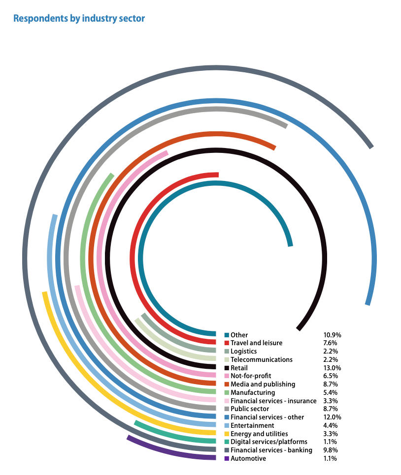{#fig-1}
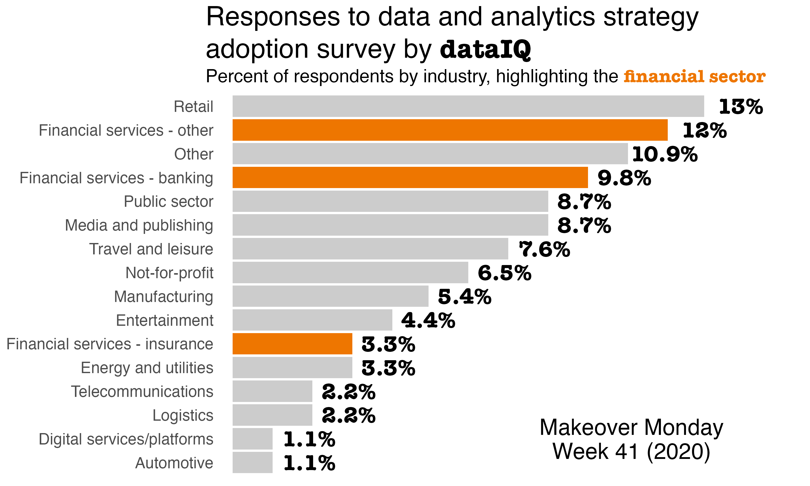{#fig-2}
# 1. Load Packages & Setup
```{r setup, include=TRUE}
if (!require("pacman")) install.packages("pacman")
pacman::p_load(
    tidyverse,
    httr,
    readxl,
    sysfonts,
    ggtext,
    janitor,   #for clean_names()
    scales,
    glue,
    here
)

font_add_google("Montserrat")
```
# 2. Read in the Data
```{r read_data, include=TRUE}
GET("https://query.data.world/s/vihrcc3hjn3umv2dy67iu2zxuyf2en", write_disk(tf <- tempfile(fileext = ".xlsx")))
df <- read_excel(tf) %>%
  clean_names()
```
# 3. Examine the Data
```{r examine, include=TRUE, echo=TRUE}
df %>%
  glimpse()
```
# 4. Tidy the Data
```{r mutate_df, include=TRUE}
financial_sector <- c('Financial services - other',
                      'Financial services - insurance',
                      'Financial services - banking')

df <- df %>%
  mutate(financial_sector =
           ifelse(industry_sector %in% financial_sector,
                  'Financial', 'Other')) %>%
  mutate(industry_sector_2 = ifelse(financial_sector == 'Financial', industry_sector, 'Other'))

industry_map <- df %>%
  select(financial_sector, industry_sector_2)
```
# 5. Visualization Parameters
```{r my_theme, include=TRUE}
mm_week <- 41
mm_year <- 2020

my_theme <- theme(
  text = element_text(family = 'Montserrat', size=12, color='black'),
  plot.title = element_textbox(),
  plot.subtitle = element_textbox(),
  axis.ticks = element_blank(),
  axis.title = element_blank(),
  axis.text.x = element_blank(),
  axis.text.y = element_text(size=14, margin = margin(r=-10)),
  plot.background = element_rect(fill = 'white'),
  panel.background =  element_blank(),
  legend.background = element_blank(),
  panel.grid.major = element_blank(),
  panel.grid.minor = element_blank(),
  panel.border = element_blank(),
  legend.title=element_blank(),
  legend.position = 'none')

industry_cols <- c('Financial' = 'darkorange2',
                   'Other' = 'gray80')
```
# 6. Plot
```{r respondents_plot, include=TRUE, fig.width=5, fig.height=3, fig.align='center'}
respondents_plot <- df %>%
  ggplot(.,
         aes(x=respondents_percent / 100,
               y=reorder(industry_sector, respondents_percent))) +
  geom_col(aes(fill=financial_sector)) +
  geom_text(aes(x=respondents_percent / 100 + .01,
                label=paste(respondents_percent, '%', sep="")),
            family='Montserrat', fontface='bold', size=7) +
  annotate("text", label="Makeover Monday\nWeek 41 (2020)", x=.11, y=2, family="Montserrat",
           size=7, lineheight=.9) +
  labs(title='Responses to data and analytics strategy adoption survey by **dataIQ**',
       subtitle=glue("Percent of respondents by industry, highlighting the <span style='color:darkorange2'>**financial sector**")) +
  scale_x_continuous(limits = c(0, .15),
                     labels = percent) +
  scale_fill_manual(values = industry_cols) +
  my_theme +
  theme(plot.title = element_textbox_simple(size=rel(2), margin = margin(b=5)),
        plot.subtitle = element_textbox_simple(size=rel(1.35), margin = margin(b=5)),
        axis.text = element_text(size=rel(1.4)))
```
# 7. Save
```{r save_plot, include=TRUE}
# Save the plot as PNG
ggsave(
  filename = glue("mm_{mm_year}_{mm_week}.png"),
  plot = respondents_plot,
  width = 10, height = 6, units = "in", dpi = 320
)

# make thumbnail for page
magick::image_read(glue("mm_{mm_year}_{mm_week}.png")) %>%
  magick::image_resize(geometry = "400") %>%
  magick::image_write(glue("mm_{mm_year}_{mm_week}_thumbnail.png"))
```
# 8. Session Info
::: {.callout-tip collapse="true"}
##### Expand for Session Info
```{r session_info, echo = FALSE}
sessionInfo()
```
:::
# 9. Github Repository
::: {.callout-tip collapse="true"}
##### Expand for GitHub Repo
[Access the GitHub repository here](https://github.com/mrafa3/mrafa3.github.io)
:::

