---
title: "How do Beyonce and Taylor Swift lyrics differ?"
description: "Using {tidytext} to process and visualize word pairs in song lyrics"
author:
- name: Mickey Rafa
url: https://mrafa3.github.io/
date: 10-04-2020
categories: [R, "#TidyTuesday", bar-plot, nlp] # self-defined categories
image: "tt_2020_40_thumbnail.png"
draft: false # setting this to `true` will prevent your post from appearing on your listing page until you're ready!
format:
html:
toc: true
toc-depth: 5
code-link: true
code-fold: true
code-tools: true
code-summary: "Show code"
self-contained: true
editor_options:
chunk_output_type: inline
execute:
error: false
message: false
warning: false
eval: true
---
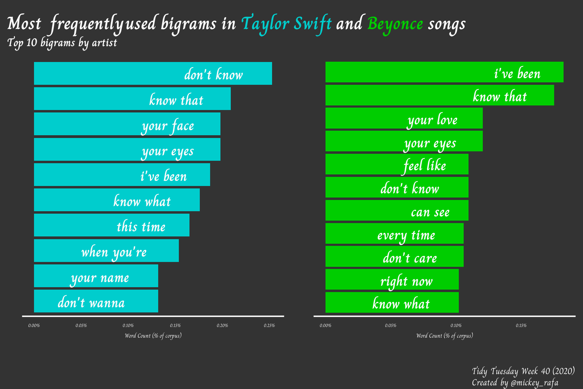{#fig-1}
# 1. Load Packages & Setup
```{r setup, include=TRUE}
if (!require("pacman")) install.packages("pacman")
pacman::p_load(
    tidyverse,
    tidytuesdayR,
    ggtext,
    showtext,
    patchwork,
    janitor,   #for clean_names()
    scales,
    htmltools, #for tagList()
    glue,
    here,
    stopwords,
    tidytext     #for text management
)

font_add_google("Charm")
showtext_auto()
```
# 2. Read in the Data
```{r read_data, include=TRUE}
tt_year <- 2020
tt_week <- 40

tuesdata <- tidytuesdayR::tt_load(tt_year, week = tt_week)

beyonce_lyrics <- tuesdata$beyonce_lyrics
taylor_swift_lyrics <- tuesdata$taylor_swift_lyrics
```
# 3. Examine the Data
```{r examine, include=TRUE, echo=TRUE}
beyonce_lyrics %>%
  glimpse()
taylor_swift_lyrics %>%
  glimpse()
```
# 4. Tidy the Data
Stop words should be approached in a custom way given the context of the data. Because lyrics tend to use lots of traditional stop words that are meaningful to the song, I chose to only filter out stop words of three characters or less (using the snowball lexicon).
```{r stop_words_lyrics, include=TRUE}
stop_words_lyrics <- stop_words %>%
  filter(lexicon == 'snowball') %>%
  filter(str_length(word) < 4)
```
I'd like to visualize the bigrams, or word pairs, in their lyrics, excluding any that are repeated words. I also considered removing any numbers, but given that I plan to only visualize the top bigrams, these won't be a factor.
```{r tok_beyonce_lyrics, include=TRUE}
tok_beyonce_lyrics <- beyonce_lyrics %>%
   janitor::clean_names() %>%
   tidytext::unnest_tokens(output = bigram,
                          input = line,
                          token = 'ngrams',
                          n = 2) %>%
   distinct(bigram, song_id, .keep_all = TRUE) %>%
   select(bigram, artist_name) %>%
   separate(bigram, into = c('first', 'second'), sep=' ', remove=FALSE) %>%
   left_join(stop_words_lyrics, by=c('first' = 'word')) %>%
   left_join(stop_words_lyrics, by=c('second' = 'word')) %>%
   mutate(first_stopword = if_else(is.na(lexicon.x), 0, 1),
          second_stopword = if_else(is.na(lexicon.y), 0, 1)) %>%
   filter(first_stopword == 0 & second_stopword == 0,
          first != second,
          !is.na(bigram)) %>%
   select(-starts_with('lexicon'),
          -ends_with('stopword')) %>%
   janitor::tabyl(bigram) %>%
   as.data.frame() %>%
   mutate(artist_name = 'Beyoncé')

tok_taylor_swift_lyrics <- taylor_swift_lyrics %>%
   janitor::clean_names() %>%
   unnest_tokens(output = bigram,
                 input = lyrics,
                 token = 'ngrams',
                 n = 2) %>%
   distinct(bigram, title, .keep_all = TRUE) %>%
   select(bigram, artist_name = artist) %>%
   separate(bigram, into = c('first', 'second'), sep=' ', remove=FALSE) %>%
   left_join(stop_words_lyrics, by=c('first' = 'word')) %>%
   left_join(stop_words_lyrics, by=c('second' = 'word')) %>%
   mutate(first_stopword = if_else(is.na(lexicon.x), 0, 1),
          second_stopword = if_else(is.na(lexicon.y), 0, 1)) %>%
   filter(first_stopword == 0 & second_stopword == 0,
          first != second) %>%
   select(-starts_with('lexicon'),
          -ends_with('stopword')) %>%
   janitor::tabyl(bigram) %>%
   as.data.frame() %>%
   mutate(artist_name = 'Taylor Swift')
```
# 5. Visualization Parameters
```{r my_theme, include=TRUE}
my_theme <- theme(
  # choose font family
  text = element_text(family = 'Charm', size=14, color='gray98'),
  axis.ticks = element_blank(),
  plot.background = element_rect(fill = "gray20", color = "gray20"),
  panel.background =  element_rect(fill = "gray20", color = "gray20"),
  panel.grid.major = element_blank(),
  panel.grid.minor = element_blank(),
  panel.border = element_blank(),
  axis.line.x = element_line(color='gray98'),
  axis.title.x = element_text(color='gray98'),
  axis.text.y = element_blank(),
  axis.text.x = element_text(color='gray98'),
  legend.position = 'none')
```
# 6. Plot
```{r tswift_viz, include=TRUE, fig.height=4, fig.width=5}
tswift_viz <- tok_taylor_swift_lyrics %>%
  slice_max(percent, n=10) %>%
  ggplot(.,
         aes(x=percent,
             y=reorder(bigram, percent))) +
  geom_col(fill = 'cyan3') +
  geom_text(aes(label = bigram),
            hjust = 1.5,
            size = 12,
            color = 'gray98',
            family = 'Charm',
            fontface = 'bold') +
  labs(x='Word Count (% of corpus)',
       y='') +
  scale_x_continuous(labels = percent) +
  my_theme

beyonce_viz <- tok_beyonce_lyrics %>%
  slice_max(percent, n=10) %>%
  ggplot(.,
         aes(x=percent,
             y=reorder(bigram, percent))) +
  geom_col(fill = 'green3') +
  geom_text(aes(label = bigram),
            hjust = 1.5,
            size = 12,
            color = 'gray98',
            family = 'Charm',
            fontface = 'bold') +
  labs(x='Word Count (% of corpus)',
       y='') +
  scale_x_continuous(labels = percent) +
  my_theme

p <- tswift_viz + beyonce_viz +
  plot_annotation(title = glue("Most frequently used bigrams in <span style='color:cyan3'>**Taylor Swift**</span> and <span style='color:green3'>**Beyonce**</span> songs"),
                  subtitle = 'Top 10 bigrams by artist',
                  caption = '<br>Tidy Tuesday Week 40 (2020)<br>Created by @mickey_rafa',
                  theme = theme(plot.title = element_textbox_simple(size=rel(4), family='Charm',
                                                                    face='bold', color='gray98',
                                                                    margin = margin(t=10)),
                                plot.subtitle = element_textbox_simple(size=rel(2.5), family='Charm',
                                                                    face='bold', color='gray98'),
                                plot.caption = element_textbox(size=rel(2), color='gray98',
                                                               family='Charm', lineheight=.3),
                                plot.background = element_rect(fill = "gray20", color = NA),
                                panel.background = element_rect(fill = "gray20"),
                                plot.margin = unit(c(0, 0, 0, 0), "pt")))
```
# 7. Save
```{r save_plot, include=TRUE}
# Save the plot as PNG
ggsave(
  filename = glue("tt_{tt_year}_{tt_week}.png"),
  plot = p,
  width = 6, height = 4, units = "in", dpi = 320
)

# make thumbnail for page
magick::image_read(glue("tt_{tt_year}_{tt_week}.png")) %>%
  magick::image_resize(geometry = "400") %>%
  magick::image_write(glue("tt_{tt_year}_{tt_week}_thumbnail.png"))
```
# 8. Session Info
::: {.callout-tip collapse="true"}
##### Expand for Session Info
```{r, echo = FALSE}
sessionInfo()
```
:::
# 9. Github Repository
::: {.callout-tip collapse="true"}
##### Expand for GitHub Repo
[Access the GitHub repository here](https://github.com/mrafa3/mrafa3.github.io)
:::
