---
title: "Analyzing size distributions in the Palmer Penguins dataset"
description: "Visualizing distributions with some alternative chart types"
author:
- name: Mickey Rafa
url: https://mrafa3.github.io/
date: 09-25-2020
categories: [R, "#TidyTuesday", ternary-plot, ridge-plot] # self-defined categories
image: "tt_2020_31_ternary_thumbnail.png"
draft: false # setting this to `true` will prevent your post from appearing on your listing page until you're ready!
format:
html:
toc: true
toc-depth: 5
code-link: true
code-fold: true
code-tools: true
code-summary: "Show code"
self-contained: true
editor_options:
chunk_output_type: inline
execute:
error: false
message: false
warning: false
eval: true
---
{#fig-1}
{#fig-2}
# 1. Load Packages & Setup
```{r setup, include=TRUE}
if (!require("pacman")) install.packages("pacman")
pacman::p_load(
    tidyverse,
    tidytuesdayR,
    dlookr,
    ggtext,
    gt,
    gtExtras,  #for font awesome icons in gt tables
    ggbump,
    showtext,
    janitor,   #for clean_names()
    scales,
    htmltools, #for tagList()
    glue,
    here,
    ggridges,
    ggtern,
    geomtextpath
)

font_add_google("Lato")
```
# 2. Read in the Data
```{r read_data, include=TRUE}
tt_year <- 2020
tt_week <- 31

tuesdata <- tidytuesdayR::tt_load(tt_year, week = tt_week)

penguins <- tuesdata$penguins
```
# 3. Examine the Data
```{r examine, include=TRUE, echo=TRUE}
penguins %>%
  glimpse()
penguins %>%
  summary()
```
# 4. Tidy the Data
```{r tidy_penguins, include=TRUE}
penguins_scale <- penguins %>%
  mutate_if(is.numeric, scale) %>%
  summarise_if(is.double, list(min, max), na.rm=TRUE)

penguins_complete <- penguins %>%
  filter(complete.cases(.))
```
# 5. Visualization Parameters
```{r my_theme, include=TRUE}
my_theme <- theme(
  text = element_text(family = 'Lato', size = 14),
  axis.ticks = element_blank(),
  plot.background = element_blank(),
  panel.background =  element_blank(),
  legend.background = element_blank(),
  panel.grid.major = element_line(colour = "grey90", linewidth = 0.5),
  panel.grid.minor = element_line(colour = "grey93", linewidth = 0.5),
  panel.border = element_blank(),
  legend.title=element_blank(),
  legend.position = 'top')

peng_cols <- c('Biscoe' = 'cornflowerblue',
                 'Dream' = 'seagreen3',
                 'Torgersen' = 'maroon1',
                 #SPECIES
                 'Adelie' = 'cornflowerblue',
                 'Chinstrap' = 'seagreen3',
                 'Gentoo' = 'maroon1')
```
# 6. Plot
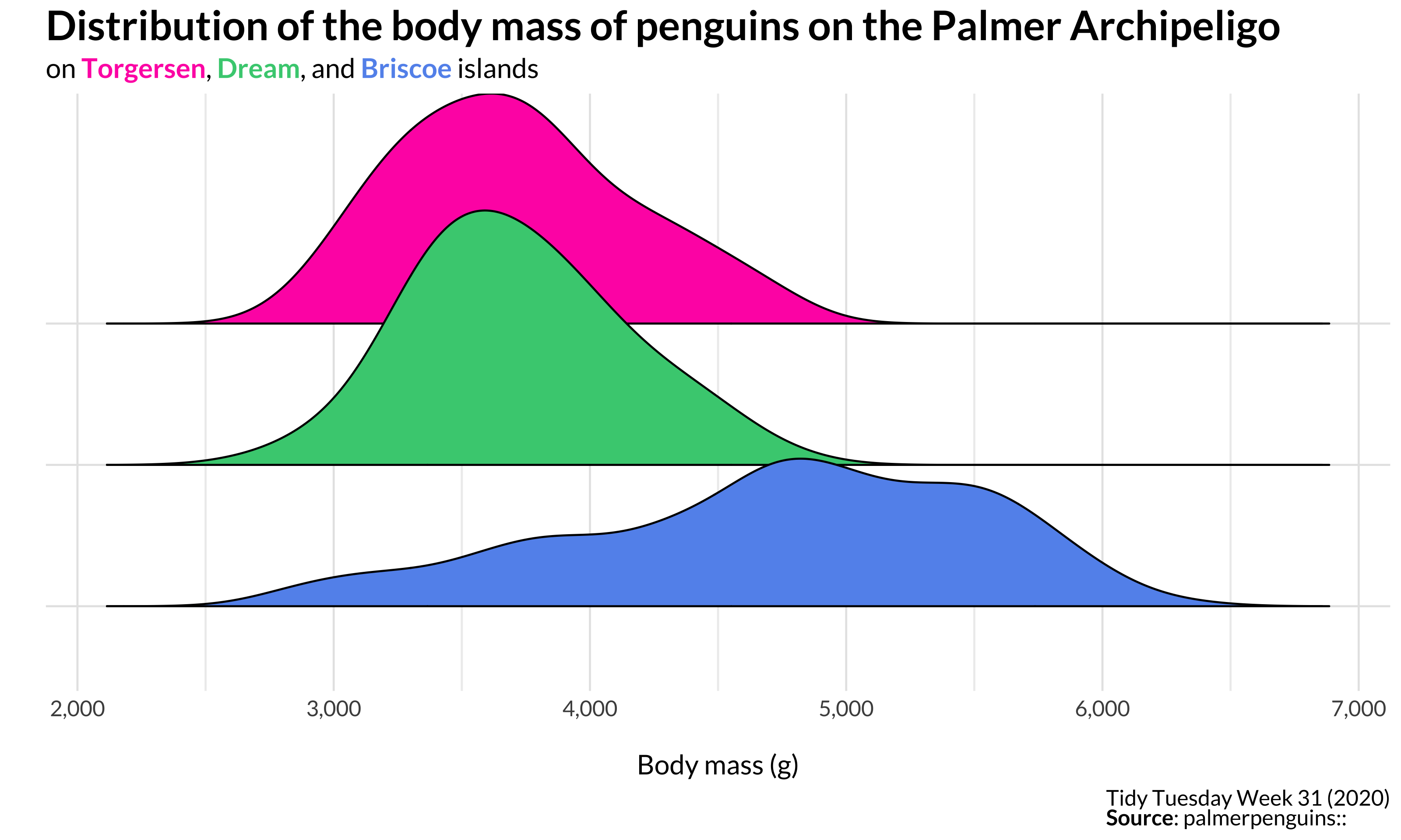
```{r pen_mass_by_island_ridgeplot_viz, include=TRUE, fig.height=6, fig.width=10}
pen_mass_by_island_ridgeplot_viz <- penguins_complete %>%
  ggplot(.) +
  ggridges::geom_density_ridges2(aes(x=body_mass_g,
                                    y=island,
                                    fill=island),
                                color='black',
                                bandwidth=195)  +
  labs(x='\nBody mass (g)',
       y='',
       title = 'Distribution of the body mass of penguins on the Palmer Archipeligo',
       subtitle = glue(
      "on <span style='color:maroon1'>**Torgersen**</span>, <span style='color:seagreen3'>**Dream**</span>, and <span style='color:cornflowerblue'>**Briscoe**</span> islands"
    ),
       caption = 'Tidy Tuesday Week 31 (2020)<br>**Source**: palmerpenguins::') +
  scale_x_continuous(labels = comma) +
  scale_fill_manual(values = peng_cols) +
  my_theme +
  theme(legend.position = 'none',
        axis.text.y = element_blank(),
        plot.title = element_text(face='bold', size=rel(1.5)),
        plot.subtitle = element_textbox(),
        plot.caption = element_textbox())
```
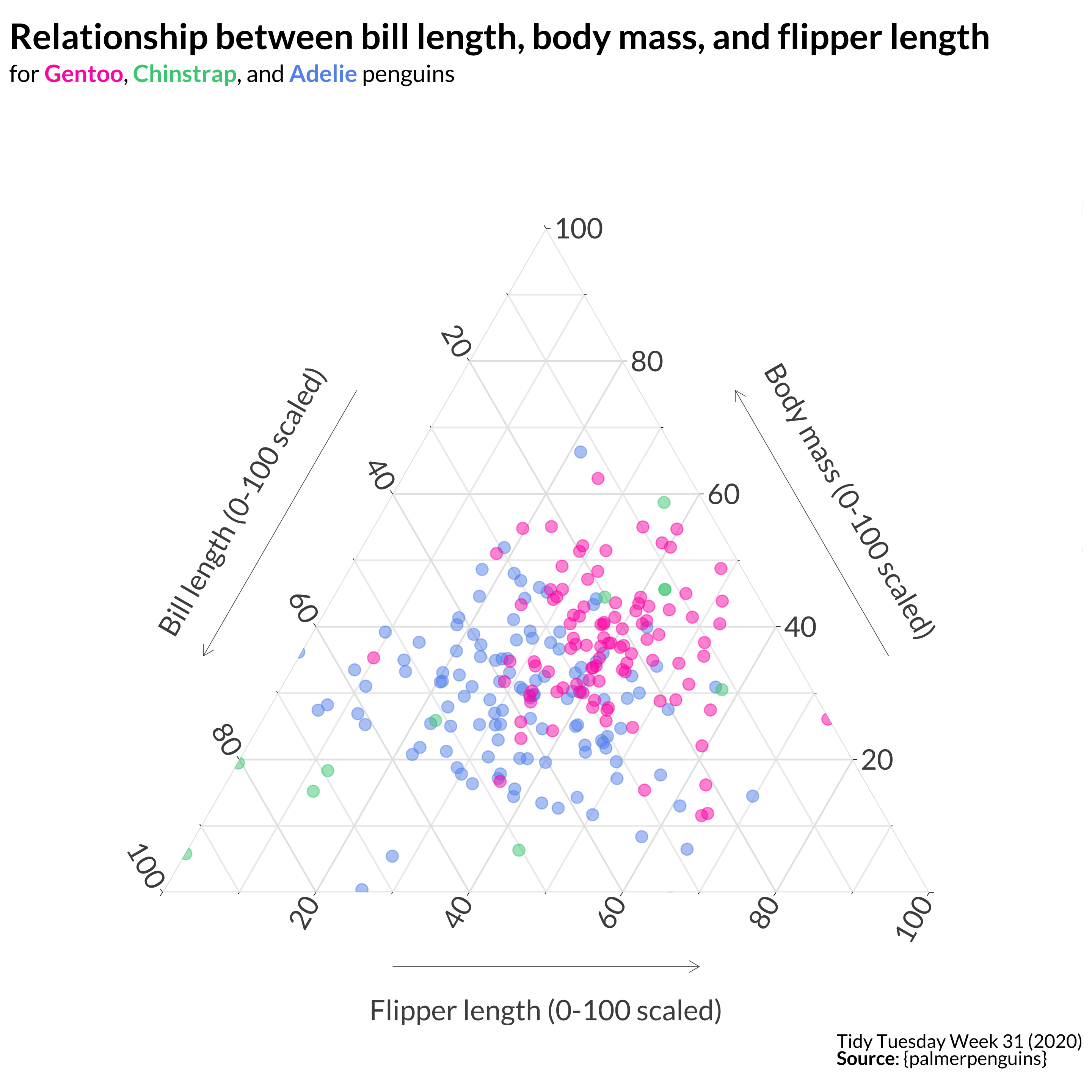
```{r penguin_ternary_viz, fig.height=9, fig.width=9}
penguin_ternary_viz <- penguins_complete %>%
  ggtern(aes(x = scale(bill_length_mm),
               y = scale(body_mass_g),
               z = scale(flipper_length_mm),
               color=species, fill=species)) +
  geom_point(aes(fill=species),
             shape = 21,
             size = 3,
             alpha = .5) +
  scale_color_manual(values = peng_cols) +
  scale_fill_manual(values = peng_cols) +
  labs(title = 'Relationship between bill length, body mass, and flipper length',
       subtitle = glue(
      "for <span style='color:maroon1'>**Gentoo**</span>, <span style='color:seagreen3'>**Chinstrap**</span>, and <span style='color:cornflowerblue'>**Adelie**</span> penguins"),
       x='', y='', z='',
      caption='Tidy Tuesday Week 31 (2020)<br>**Source**: {palmerpenguins}') +
  Larrowlab("Bill length (0-100 scaled)\n") +
  Tarrowlab("Body mass (0-100 scaled)\n") +
  Rarrowlab("\nFlipper length (0-100 scaled)") +
  my_theme +
  theme(tern.axis.arrow.show = TRUE,
        plot.title = element_text(face='bold', size=rel(1.5), lineheight = 1.5),
        tern.axis.text = element_text(size = rel(1.5)),
        legend.position = 'none',
        plot.subtitle = element_textbox(),
        plot.caption = element_textbox())
```
# 7. Save
```{r save_plot, include=TRUE}
# RIDGEPLOT
ggsave(
  filename = glue("tt_{tt_year}_{tt_week}_ridge.png"),
  plot = pen_mass_by_island_ridgeplot_viz,
  width = 10, height = 6, units = "in", dpi = 320
)

# make thumbnail for page
magick::image_read(glue("tt_{tt_year}_{tt_week}_ridge.png")) %>%
  magick::image_resize(geometry = "400") %>%
  magick::image_write(glue("tt_{tt_year}_{tt_week}_ridge_thumbnail.png"))

# TERNARY
ggsave(
  filename = glue("tt_{tt_year}_{tt_week}_ternary.png"),
  plot = penguin_ternary_viz,
  width = 9, height = 9, units = "in", dpi = 320
)

# make thumbnail for page
magick::image_read(glue("tt_{tt_year}_{tt_week}_ternary.png")) %>%
  magick::image_resize(geometry = "400") %>%
  magick::image_write(glue("tt_{tt_year}_{tt_week}_ternary_thumbnail.png"))
```
# 8. Session Info
::: {.callout-tip collapse="true"}
##### Expand for Session Info
```{r, echo = FALSE}
sessionInfo()
```
:::
# 9. Github Repository
::: {.callout-tip collapse="true"}
##### Expand for GitHub Repo
[Access the GitHub repository here](https://github.com/mrafa3/mrafa3.github.io)
:::

