Analysis of Gapminder data using nested models in R

Working on nesting models following the workflow from R for Data Science.

        country        continent        year         lifeExp     
 Afghanistan:  12   Africa  :624   Min.   :1952   Min.   :23.60  
 Albania    :  12   Americas:300   1st Qu.:1966   1st Qu.:48.20  
 Algeria    :  12   Asia    :396   Median :1980   Median :60.71  
 Angola     :  12   Europe  :360   Mean   :1980   Mean   :59.47  
 Argentina  :  12   Oceania : 24   3rd Qu.:1993   3rd Qu.:70.85  
 Australia  :  12                  Max.   :2007   Max.   :82.60  
 (Other)    :1632                                                
      pop              gdpPercap       
 Min.   :6.001e+04   Min.   :   241.2  
 1st Qu.:2.794e+06   1st Qu.:  1202.1  
 Median :7.024e+06   Median :  3531.8  
 Mean   :2.960e+07   Mean   :  7215.3  
 3rd Qu.:1.959e+07   3rd Qu.:  9325.5  
 Max.   :1.319e+09   Max.   :113523.1

#create year_since_1950
gapminder <- gapminder %>% 
  mutate(year_since_1950 = year - 1950)
#group by data that you want to produce multiple models by
#then nest to create data column of remaining columns
nest_gapminder <- gapminder %>% 
  group_by(continent, country) %>% 
  nest()

#create function for model that you want to build
#df will be the only parametre
continent_year_model <- function(df) {
  lm(lifeExp ~ year_since_1950, data = df)
}

#take nested df and map function to the data column
#model will keep nested model statistics by country/year
nest_gapminder <- nest_gapminder %>% 
  mutate(model = map(data, continent_year_model),
         glance = map(model, broom::glance))

glance_gapminder_model <- nest_gapminder %>% 
  unnest(glance) %>% 
  arrange(desc(adj.r.squared))

glance_gapminder_model %>% 
  ggplot(.) + 
  geom_jitter(aes(x=continent,
                 y=r.squared,
                 color=continent)) + 
  ggtitle('Distribution of model fit by continent',
          subtitle = 'Each dot is a country model') + 
  labs(x='Continent',
       y='R-squared',
       caption='LifeExp ~ year') + 
  my.theme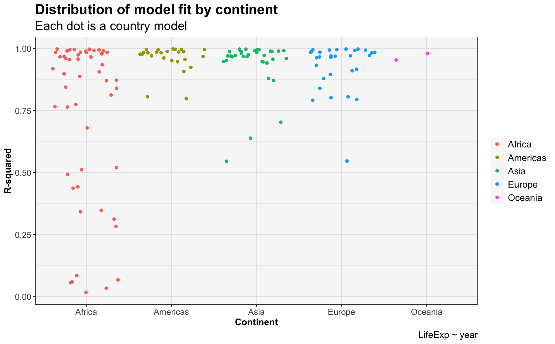

glance_gapminder_model %>% 
  ggplot(.) + 
  geom_density_ridges(aes(x=r.squared, 
                          y=continent,
                          fill=continent)) + 
  ggtitle('Distribution of model fits by continent',
          subtitle = 'Time does not explain variance in African life expectancy as strongly as others') + 
  labs(x='R-squared',
       y='Continent',
       caption='LifeExp ~ year') + 
  my.theme

Picking joint bandwidth of 0.0392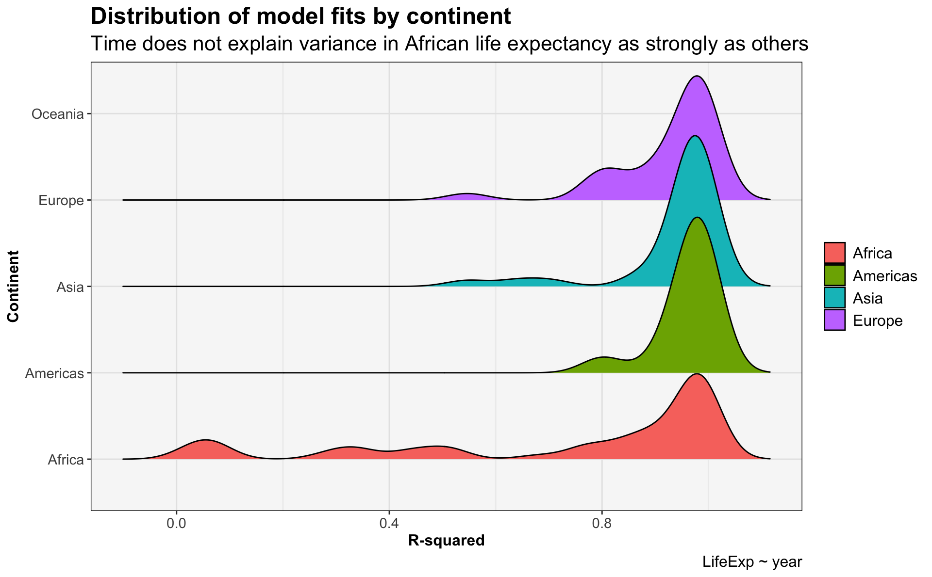

#which countries have the poor fits?
bad_fit <- glance_gapminder_model %>% filter(r.squared < 0.4)

gapminder %>% 
  semi_join(bad_fit, by = "country") %>% 
  ggplot(.) + 
    geom_line(aes(x=year, 
                  y=lifeExp, 
                  color=country), linewidth=1.1) + 
  ggtitle('Countries in which time does not adequately explain life expectancy',
          subtitle = 'Visualizing countries with model fits less than .4') + 
  labs(x='Year',
       y='Life expectancy',
       caption='LifeExp ~ year') + 
  my.theme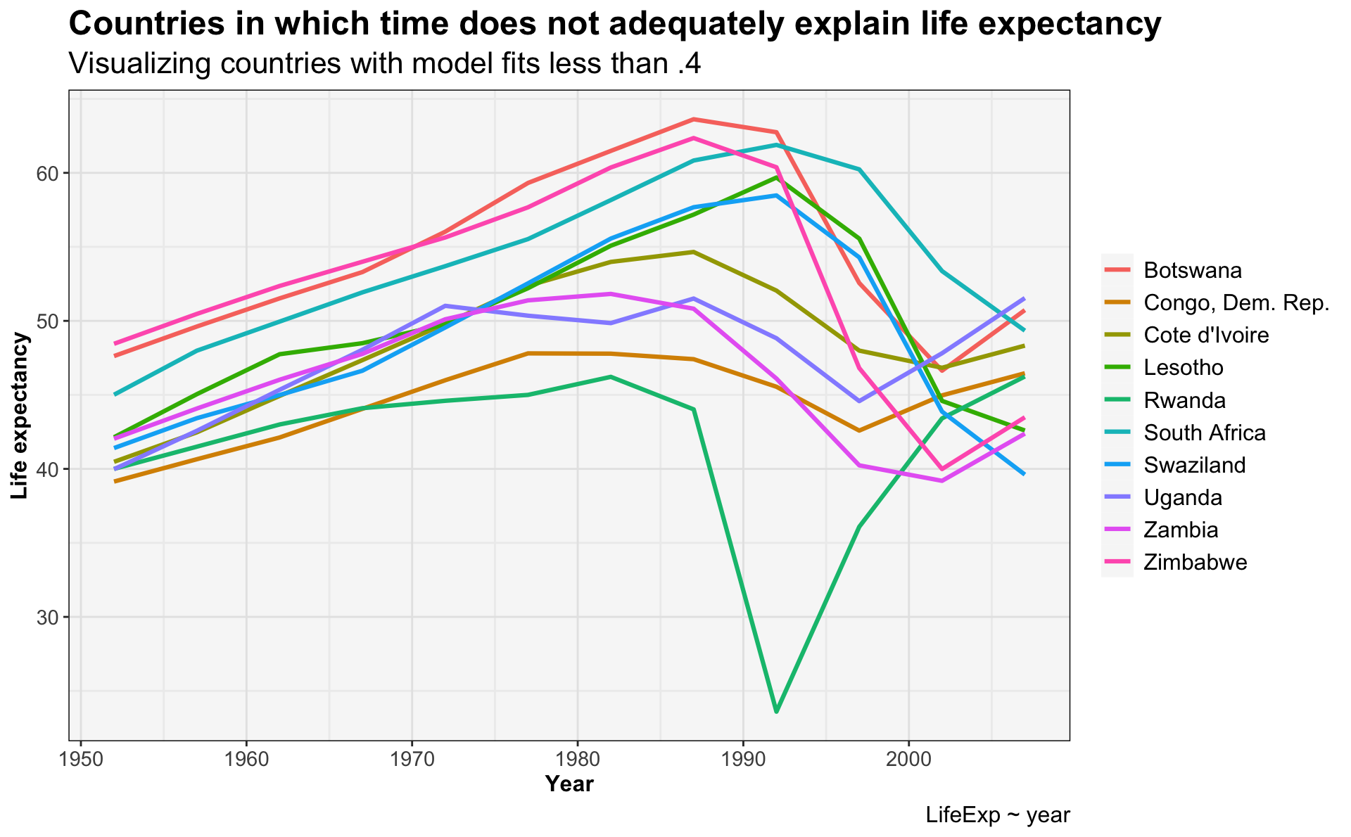

This demonstrates that:

The 10 countries with the poorest model fits are all in Africa.
The fit seems to be due to a dramatic decline in life expectancy that begins around 1990. This is the HIV/AIDS epidemic.
From R for Data Science (http://r4ds.had.co.nz/many-models.html#making-tidy-data-with-broom):

Making tidy data with broom:

The broom package provides three general tools for turning models into tidy data frames:

broom::glance(model) returns a row for each model. Each column gives a model summary: either a measure of model quality, or complexity, or a combination of the two.
broom::tidy(model) returns a row for each coefficient in the model. Each column gives information about the estimate or its variability.
broom::augment(model, data) returns a row for each row in data, adding extra values like residuals, and influence statistics.